Introduction
In the last few sections, we've talked about types of market failure, situations in which the unregulated market fails to produce where MSB = MSC. We've relatively loosely thrown around the idea that the government can take action in markets, but we haven't looked super closely into how the government actually does so (outside of our short discussion of Pigouvian taxes and subsidies). This guide will look at two main tools of government intervention in markets: taxes/subsidies and price controls, specifically in relation to regulating a monopoly.

Effects of Per-Unit and Lump Sum Taxes on Cost Curves
The main action of the government is to either tax firms, forcing them to give money to the government, or subsidize firms, giving them money. We talked about excise taxes on markets back in unit 2, but haven't looked deep into how per-unit and lump sum taxes impact the firm.
Per-Unit vs. Lump Sum Taxes
First, let's break down the difference between a per-unit tax and a lump sum tax. A per-unit tax is exactly what it sounds like: a smaller tax on every unit produced. For example, suppose for every laptop produced by Apple, $2 had to go to the government. This is a per-unit tax. By contrast, a lump sum tax is a one time fixed tax. For example, if the government taxed Apple a flat $500.
This is an important distinction because this means a lump sum tax is in essence a fixed cost, whereas a per-unit tax impacts marginal cost.
Graphing Taxes in the Firm
This guide will focus on graphing taxes since that's most common, but graphing a subsidy is the exact same just in the opposite direction. We'll also assume a perfectly competitive market for simplicity, but the same applies for a Monopoly/Monopolistic Competition since MC and ATC are the same in either market.
Per-Unit Taxes
A per-unit tax is in essence an addition to marginal cost, since it is an additional cost on every additional unit. For example, if producing every additional unit was $3 and we applied a $1 per unit tax, marginal cost is now 4. The original 3 plus the tax of 1. Thus, marginal cost will shift up with a per-unit tax. Along with marginal cost, ATC will shift up as well. This is because a per-unit tax impacts variable costs and thus ATC.
This is visualized in the graph below:
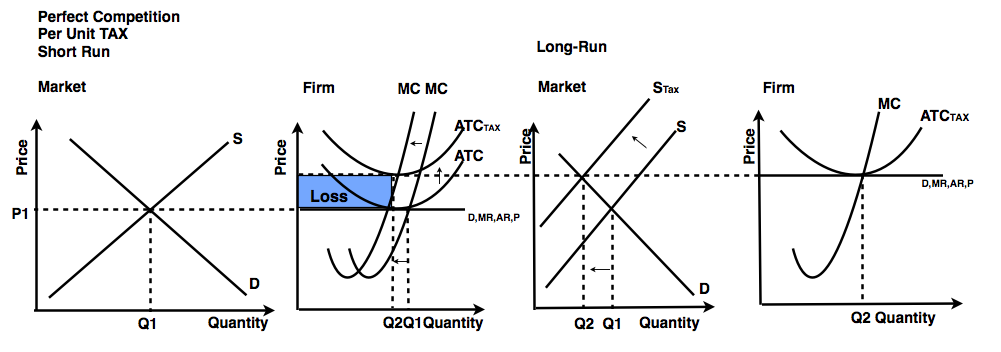
In this graph, we see the shift left of MC and the shift up of ATC, leading to a loss in the market. We also see a reminder of the long-run adjustment that would happen with a perfectly competitive market.
Lump Sum Taxes
Unlike a per-unit tax, a lump sum tax does not affect marginal cost. This is because it is a one time fixed tax. This means it shifts AFC and ATC up (but we usually don't draw AFC, so just ATC in most cases). Once again, this graph shows us the long-run adjustment as well:

Regulating a Monopoly
A monopoly, as mentioned in Unit 4, is a market where the most efficient number of firms in the industry is only one. Here's the graph for a monopoly:
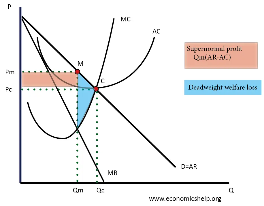
Point M is where a monopoly would produce when they are unregulated by the government. At this point, we have a pretty large area of deadweight loss, meaning we have some degree of market failure, where we are not allocating resources to the point where P = MC.
We have a few different places we can regulate a monopoly to avoid this. In particular, the socially optimal point and the fair-return point.
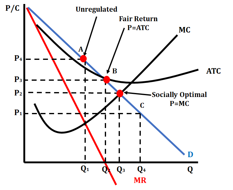
The most obvious approach is to set a price ceiling at P2 in the above graph to force the monopoly to produce at P2 and Q3, the socially optimal price and quantity. However, there's a problem: the firm's making a loss! The monopoly will need a lump-sum subsidy to produce here. This will cause ATC to shift down to the point where the firm will break even at the socially optimal point.
Another option is to simply compromise with the monopoly and let it produce where they break even, at point B in the above graph. At this point, P3 and Q2, the firm makes zero profit, but the government also doesn't have to subsidize the firm. There is a small amount of deadweight loss (see if you can spot it!), but much less than before.
Frequently Asked Questions
What's the difference between a per-unit tax and a lump-sum tax and when do I use each one?
A per-unit tax is a tax charged on each unit sold (e.g., $1 per widget). It raises firms’ marginal cost, shifts the supply curve up/left, lowers equilibrium quantity, raises the price consumers pay, reduces producer price received, creates deadweight loss, and generates government revenue. The incidence depends on price elasticities of demand and supply (CED EK POL-4.A.1). Use per-unit taxes/subsidies in problems where quantity and welfare (CS, PS, DWL, revenue) change and you’ll usually show it on supply/demand or firm graphs and calculate new equilibria. A lump-sum (fixed) tax is a one-time or per-period fixed charge independent of output. It raises firms’ fixed costs/average total cost but does NOT change marginal cost or the profit-maximizing output; it affects profits but not quantity, consumer/producer surplus, or DWL (EK POL-4.A.2). Lump-sum subsidies are the tool for natural monopolies to reach allocative efficiency without changing MC (EK POL-4.A.6). For AP free-response, be ready to show these effects on graphs and compute changes (see the Unit 6 study guide: https://library.fiveable.me/ap-microeconomics/unit-6/effects-government-intervention-different-market-structures/study-guide/Vo9KNzD2qK0rP6aGQkhe). For extra practice, try problems at https://library.fiveable.me/practice/ap-microeconomics.
How do I know if a price ceiling will actually affect the market or not?
Check the ceiling vs the market price you’d get without policy. If the ceiling is below the equilibrium (or below the market price a monopoly chooses), it’s binding and will change outcomes; if it’s at or above equilibrium (or above the monopoly price) it’s non-binding and does nothing. In perfect competition: ceiling < equilibrium price → price forced down, quantity demanded > quantity supplied (shortage). In monopoly or imperfect markets: compare the ceiling to the firm’s chosen price (where MR = MC); if the ceiling is above that price it won’t bind (EK POL-4.A.3, EK POL-4.A.5). Remember elasticity matters: more elastic supply/demand means larger quantity responses and different consumer/producer surplus and deadweight loss (EK POL-4.A.1). On the AP exam you should show this with well-labeled graphs (free-response Skill 4 tasks). For extra practice and visuals, see the Topic 6.4 study guide (https://library.fiveable.me/ap-microeconomics/unit-6/effects-government-intervention-different-market-structures/study-guide/Vo9KNzD2qK0rP6aGQkhe) and unit review (https://library.fiveable.me/ap-microeconomics/unit-6).
I'm confused about deadweight loss - why does government intervention sometimes create it and sometimes reduce it?
Deadweight loss (DWL) is simply the lost surplus from trades that no longer happen. Government intervention creates DWL when it moves quantity away from the allocatively efficient level (where P = MC). Examples: a per-unit tax raises consumer price and lowers quantity → fewer mutually beneficial trades → DWL (size depends on demand/supply elasticities). A binding price ceiling or floor in a competitive market also reduces traded quantity and creates DWL. But intervention can reduce DWL when it fixes a market failure that already caused inefficient quantity. Examples: regulating a monopoly price toward marginal-cost pricing or using antitrust to increase competition raises quantity toward the social optimum and cuts the monopoly DWL (CED EK POL-4.A.5, EK POL-4.A.4). A lump-sum subsidy to a natural monopoly can allow production at the allocatively efficient quantity without changing MC (EK POL-4.A.6). For AP free-response you’ll need correctly labeled graphs and calculations showing changes in CS, PS, government revenue/cost, and DWL (Topic 6.4 study guide: https://library.fiveable.me/ap-microeconomics/unit-6/effects-government-intervention-different-market-structures/study-guide/Vo9KNzD2qK0rP6aGQkhe; unit overview: https://library.fiveable.me/ap-microeconomics/unit-6). Practice problems: https://library.fiveable.me/practice/ap-microeconomics.
Can someone explain how price elasticity affects who pays more of a per-unit tax?
Who pays more of a per-unit tax depends on relative price elasticities of demand and supply (EK POL-4.A.1). The side that’s more inelastic (less responsive to price) will bear a larger share of the tax. Why: with an inelastic demand, consumers don’t reduce quantity much when price rises, so sellers can pass most of the tax onto buyers as a higher price. With inelastic supply, producers can’t easily cut quantity, so they absorb more of the tax as a lower net price received. Quick example: if demand is very inelastic (|εd| = 0.2) and supply is elastic (εs large), consumers pay almost the whole tax. If supply is inelastic and demand elastic, producers pay most. On the AP exam you should be able to show this with a correctly labeled supply/demand graph (shift supply up by the tax, show consumer price, producer net price, changes in consumer/producer surplus and deadweight loss)—see the Topic 6.4 study guide for graphs and practice (https://library.fiveable.me/ap-microeconomics/unit-6/effects-government-intervention-different-market-structures/study-guide/Vo9KNzD2qK0rP6aGQkhe). For extra practice, try problems at the unit page (https://library.fiveable.me/ap-microeconomics/unit-6) or the practice bank (https://library.fiveable.me/practice/ap-microeconomics).
What happens to consumer and producer surplus when the government puts a subsidy on a monopoly?
A per-unit subsidy to a monopoly lowers the firm’s marginal cost (MC) by the subsidy amount, shifting MC down. The monopolist then sets output where MR = new MC, so quantity rises and the monopoly price falls. Consumer surplus increases (more quantity and lower price). Producer surplus usually increases too because the firm now gets a lower cost plus a subsidy per unit, raising profit—so producers capture part of the subsidy. Deadweight loss from monopoly shrinks because output moves closer to the allocatively efficient Q (P = MC), though DWL only disappears if the subsidy is exactly large enough to make price = true marginal cost. Note: a lump-sum subsidy wouldn’t change MC or Q (EK POL-4.A.2). Be ready to show this on the AP free-response graph (MR, MC, demand; label changes)—see the Topic 6.4 study guide for visuals and practice (https://library.fiveable.me/ap-microeconomics/unit-6/effects-government-intervention-different-market-structures/study-guide/Vo9KNzD2qK0rP6aGQkhe). For more practice, try problems at (https://library.fiveable.me/practice/ap-microeconomics).
How do I calculate the change in government revenue from a per-unit tax using a supply and demand graph?
Put the tax on your graph as a vertical distance t between the original supply and the new (supplier’s) curve. The tax raises the price consumers pay (Pc) and lowers the price producers receive (Pp); Pc − Pp = t. Find the new equilibrium quantity Q* where demand intersects the taxed supply. Government revenue = tax per unit × quantity sold with the tax = t × Q*. Example: if the per-unit tax is $2 and the new equilibrium quantity from the graph is 50 units, revenue = $2 × 50 = $100. Remember elasticity matters: a more elastic demand or supply gives a bigger Q drop and lowers revenue. This is exactly EK POL-4.A.1 territory—on the AP free-response you may be asked to compute revenue from numbers read off a graph or table (so show Pc, Pp, t, and Q*). For quick review, see the Topic 6.4 study guide (https://library.fiveable.me/ap-microeconomics/unit-6/effects-government-intervention-different-market-structures/study-guide/Vo9KNzD2qK0rP6aGQkhe) and more practice at (https://library.fiveable.me/practice/ap-microeconomics).
Why would a natural monopoly need a lump-sum subsidy to be allocatively efficient?
A natural monopoly has falling average total cost (big fixed cost, low MC), so the allocatively efficient rule (P = MC) would set price below average total cost—the firm would lose money. A per-unit subsidy that raises MC-based net price would change marginal cost incentives and distort output. A lump-sum subsidy covers the firm’s fixed costs without changing its marginal cost curve (EK POL-4.A.2), so the firm can set P = MC, produce the allocatively efficient quantity, and remain financially viable. That’s why AP CED says a natural monopoly requires a lump-sum subsidy to achieve allocative efficiency (EK POL-4.A.6). For the exam, be ready to show this on a graph: MC, ATC, demand, label P = MC output, and show the subsidy shifting ATC down via fixed-cost coverage. See the Topic 6.4 study guide for a refresher (https://library.fiveable.me/ap-microeconomics/unit-6/effects-government-intervention-different-market-structures/study-guide/Vo9KNzD2qK0rP6aGQkhe) and grab practice problems at (https://library.fiveable.me/practice/ap-microeconomics).
I don't understand the difference between how price floors work in perfect competition vs monopoly markets - help?
Short version: a binding price floor forces price above the market-clearing level. In perfect competition that creates excess supply (a surplus): quantity supplied rises, quantity demanded falls, firms individually are price takers so each sells at the floor price; consumer surplus falls, producer surplus may rise for some units but total surplus falls and deadweight loss appears. If the government buys the surplus, it pays the gap (gov’t spending). In a monopoly, a price floor can have a very different effect. A monopoly sets MR = MC to pick Q and then charges the corresponding demand price. If you set a floor above the monopoly price but below the monopolist’s profit-maximizing price, the monopolist might be forced to increase output (if Pfloor > monopoly price at MR=MC) up to where Pfloor = demand for that Q—which can increase output toward the allocatively efficient level and reduce deadweight loss (price regulation can improve efficiency: EK POL-4.A.5). If the floor is above what demand will buy at any profit-maximizing behavior, it may simply be nonbinding. For AP exam answers: draw labeled graphs (perfect competition: supply & demand + surplus areas; monopoly: demand, MR, MC, show new P and Q) and calculate changes in CS, PS, DWL. Review the Topic 6.4 study guide (https://library.fiveable.me/ap-microeconomics/unit-6/effects-government-intervention-different-market-structures/study-guide/Vo9KNzD2qK0rP6aGQkhe) and practice problems (https://library.fiveable.me/practice/ap-microeconomics) for graph practice.
What's the point of antitrust policy and how does it actually make markets more competitive?
Antitrust policy exists to stop firms from using market power to raise price and restrict output—so markets work more like competitive ones (CED EK POL-4.A.7). In practice regulators block anticompetitive mergers, break up firms, punish collusion, or force rules that lower barriers to entry. That increases the number of sellers, pushes price down toward marginal cost, raises quantity, increases consumer surplus, and shrinks deadweight loss (you’d show this on a price/quantity graph: monopoly P > MC and Q < socially efficient Q). Note: natural monopolies are different—price regulation or a lump-sum subsidy is often needed for allocative efficiency (EK POL-4.A.6). For AP: be ready to explain these effects with a graph and calculate changes in surplus/quantity (Topic 6.4). For more review and practice, see the Topic 6.4 study guide (https://library.fiveable.me/ap-microeconomics/unit-6/effects-government-intervention-different-market-structures/study-guide/Vo9KNzD2qK0rP6aGQkhe), the Unit 6 overview (https://library.fiveable.me/ap-microeconomics/unit-6), and extra practice problems (https://library.fiveable.me/practice/ap-microeconomics).
How do I show on a graph that government intervention is actually increasing efficiency instead of decreasing it?
Show it by drawing before-and-after graphs and comparing deadweight loss (DWL). On your original graph, label demand (MB), supply or MC, and the monopoly MR and MC if it’s imperfect competition. Mark the initial outcome and the allocatively efficient quantity where P = MC. If government policy (price regulation, per-unit subsidy, lump-sum subsidy for a natural monopoly, or antitrust) moves quantity closer to that P = MC point, shade the DWL triangle before and after—efficiency rises when that triangle shrinks or disappears. Also show changes in consumer and producer surplus and any government revenue/cost (for a per-unit subsidy, include government cost). For monopolies note EK POL-4.A.5–6: price-regulation that sets P≈MC increases allocative efficiency; natural monopolies need a lump-sum subsidy to hit the efficient Q. On the AP FRQ, draw and label both graphs and compute/compare areas (surpluses and DWL). For a quick review, see the Topic 6.4 study guide (https://library.fiveable.me/ap-microeconomics/unit-6/effects-government-intervention-different-market-structures/study-guide/Vo9KNzD2qK0rP6aGQkhe) and practice problems (https://library.fiveable.me/practice/ap-microeconomics).
When does a binding price ceiling cause shortages in a monopoly market compared to a perfectly competitive market?
Short answer: A binding price ceiling causes shortages in perfect competition whenever it’s set below the market equilibrium price—price < Pe makes Qd > Qs, so a shortage appears (textbook supply–demand result; EK POL-4.A.3). In a monopoly the story’s a bit different. A ceiling only binds if it’s below the monopolist’s chosen price. If it’s below that price, the monopolist will raise output (because it can’t charge its old price) to the point where MR = MC subject to the new price or until demand at the ceiling price determines Q. A shortage occurs only if the quantity that consumers want at the ceiling price exceeds the quantity the monopolist is willing/able to supply at that price. So: ceiling < monopoly price → may increase Q but may or may not create a shortage; ceiling below the competitive (allocatively efficient) price will definitely cause excess demand. (See EK POL-4.A.5 and POL-4.A.3.) For a clear graphed explanation and practice problems, check the Topic 6.4 study guide (https://library.fiveable.me/ap-microeconomics/unit-6/effects-government-intervention-different-market-structures/study-guide/Vo9KNzD2qK0rP6aGQkhe) and more unit review/practice at (https://library.fiveable.me/ap-microeconomics/unit-6) and (https://library.fiveable.me/practice/ap-microeconomics).
Can you explain why lump-sum taxes don't affect marginal cost but per-unit taxes do?
A lump-sum tax is a fixed cost paid regardless of output, so it raises a firm’s total and average fixed cost but does not change the cost of producing one more unit. Marginal cost (MC) is the extra cost of one additional unit—because the lump sum doesn’t vary with output, MC stays the same. A per-unit tax (specific tax) adds the same extra cost to each unit produced, so it raises MC by that tax amount at every output level. On graphs, a lump-sum tax shifts ATC up (worse profits) but leaves MC and the firm’s output rule (P = MC in perfect competition) unchanged; a per-unit tax shifts both MC and supply up/left, reducing equilibrium quantity and changing prices, surpluses, deadweight loss, and government revenue (EK POL-4.A.1 and EK POL-4.A.2). For practice drawing these shifts (required on AP free-response), see the Topic 6.4 study guide (https://library.fiveable.me/ap-microeconomics/unit-6/effects-government-intervention-different-market-structures/study-guide/Vo9KNzD2qK0rP6aGQkhe) and try related problems (https://library.fiveable.me/practice/ap-microeconomics).
What's the difference between allocative efficiency and productive efficiency when talking about government regulation of monopolies?
Allocative efficiency means producing the quantity where price = marginal cost (P = MC) so that marginal benefit to consumers equals marginal cost of production—no deadweight loss. Productive efficiency means producing at the lowest possible average total cost (output at minimum ATC). For monopolies: an unregulated monopoly is allocatively and productively inefficient (it sets P > MC and usually doesn’t produce at min ATC). Policy choices trade off these goals: forcing price down to P = MC restores allocative efficiency but may make a natural monopoly incur losses (so the government may need a lump-sum subsidy—EK POL-4.A.6). Setting price = ATC (average-cost pricing) prevents losses (zero economic profit) but is not allocatively efficient (P > MC). On the AP free-response you’ll often need the graphs and calculations showing these outcomes (see Topic 6.4 study guide for examples) (https://library.fiveable.me/ap-microeconomics/unit-6/effects-government-intervention-different-market-structures/study-guide/Vo9KNzD2qK0rP6aGQkhe). For extra practice, use Fiveable’s unit review and practice questions (https://library.fiveable.me/ap-microeconomics/unit-6; https://library.fiveable.me/practice/ap-microeconomics).
How do I know if government intervention is fixing market failure or just creating more problems?
Ask: does policy move the market toward the social optimum or away from it? If it reduces deadweight loss and aligns private incentives with social costs/benefits, it’s fixing market failure (EK POL-4.A.4). Check on a graph: does quantity move closer to the allocatively efficient Q* and does total surplus (consumer + producer + government where relevant) rise? Use the CED tools: measure changes in consumer/producer surplus, government revenue/cost, and deadweight loss for per-unit taxes/subsidies (EK POL-4.A.1), price controls (EK POL-4.A.3), or subsidies/taxes for natural monopoly (EK POL-4.A.6). Watch for wrong incentives: policies that create larger DWL, persistent shortages/surpluses, or make firms worse off without addressing externalities are creating problems. Don’t forget elasticity—impacts depend on price elasticities (EK POL-4.A.1). Practice drawing labeled graphs (Skill 4) and doing calculations from the CED. Review the Topic 6.4 study guide (https://library.fiveable.me/ap-microeconomics/unit-6/effects-government-intervention-different-market-structures/study-guide/Vo9KNzD2qK0rP6aGQkhe) and try more practice problems (https://library.fiveable.me/practice/ap-microeconomics).
I'm studying for the FRQ and need to know how to calculate the deadweight loss from a price floor in different market structures.
Quick method you can use on FRQs: draw the market, label the equilibrium (Pe, Qe) and the binding floor (Pf > Pe). Find the new quantity traded (Qt)—with a price floor that’s enforced and government buys the surplus, Qt is the quantity demanded at Pf. Deadweight loss (DWL) is the triangular loss of mutually beneficial trades between Qt and Qe. Formula (works for any market): DWL = 1/2 × (Qe − Qt) × [Pd(Qt) − Ps(Qt)] - Qe = equilibrium quantity before the floor. - Qt = quantity actually traded after the floor (quantity demanded at Pf). - Pd(Qt) = value buyers place at Qt (the demand price at Qt; often equals Pf). - Ps(Qt) = cost to sellers at Qt (the supply price / marginal cost at Qt). Example: Pe = $5, Qe = 100; Pf = $7 → Qt = 80. If sellers’ marginal cost at Q = 80 is $4, Pd(Qt)=7, Ps(Qt)=4: DWL = 0.5 × (100−80) × (7−4) = 0.5 × 20 × 3 = $30. Notes for different market structures: - Perfect competition: use supply = MC for Ps(Qt). Government purchases may create surplus; use the formula above. (CED EK POL-4.A.3, A.1) - Monopoly/monopolistic competition: recalc Qt from the firm’s profit-maximizing condition (MR = MC) given the regulated price. If the floor is below monopoly price it’s nonbinding (no effect). If it’s binding, Qt is where demand at Pf intersects quantity the firm chooses (or where MR=MC if firm still restricts output); use the same DWL triangle but Ps(Qt) is the firm’s marginal cost at Qt. - Monopsony: a binding minimum wage (floor) can increase quantity and reduce DWL; still compute area between demand and supply (or VMPL and MCL). On the exam: draw accurate graphs and show your algebra/area work (Skill 4 and numerical analysis requirements). For more worked examples and practice, see the Topic 6.4 study guide (https://library.fiveable.me/ap-microeconomics/unit-6/effects-government-intervention-different-market-structures/study-guide/Vo9KNzD2qK0rP6aGQkhe) and try problems at (https://library.fiveable.me/practice/ap-microeconomics). Fiveable’s guides are aligned to the CED so they’re handy for FRQ prep.