Factor Supply and Demand
In a factor market, the roles of supplier and demander are flipped. Instead of consumers demanding products supplied by producers, producers demand labor supplied by consumers. However, the laws of supply and demand still apply to factor markets. Let's break down each part of the market:

Factor Supply
Factor supply, also written in AP Micro as labor supply (since unit 5 focuses on factors broadly but specifies mostly on labor, not capital), is the non-firm side of a factor market. Labor supply represents the lowest willingness and ability to sell one's labor to a firm. Factor supply follows the traditional law of supply: as quantity increases, wage increases. This is because with a higher wage, people are willing to supply more labor. This is fairly intuitive. If you were paid $50/hour to study for AP Micro, you'd probably study a bit more for AP Micro. But you love AP Micro, so you're studying with us for free! You do love AP Micro...right?
Economists Being Economists Moment: You may notice that Labor is notated as "N" in the graphs below. This is because economists use the letter "N" to mean labor. You can also use L in AP Micro! So LD and LS are acceptable.
Factor Demand
Factor demand works almost exactly analogously to how product demand worked in unit 2 of AP Micro. At a high wage, firms are not willing to buy much labor, and at a low wage, firms are willing to buy more labor. This leads to a downward sloping demand curve for labor.
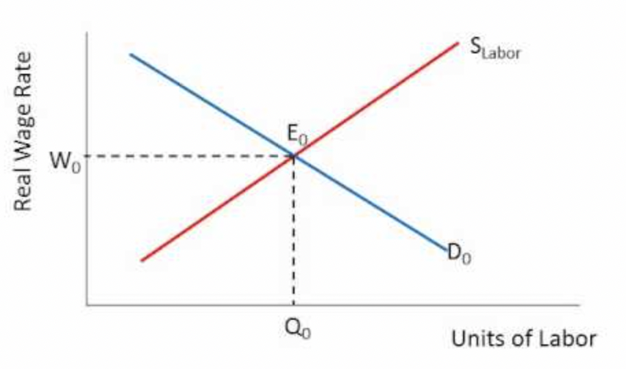
Factor Market Equilibrium
Like a normal market, the market labor and wage rate are set at the point where the quantity of labor supplied equals the quantity of labor demanded. At this point, all workers who are willing and able to sell their labor do so to firms that are willing and able to hire them. There is no shortage of workers or surplus of labor.
Shortages and Surpluses of Labor
If the price in a labor market is above or below the equilibrium price, the market will experience either a shortage or surplus of labor. This is basically the same as unit 2's surpluses and shortages.
Below is a surplus of labor caused by an artificially high wage. This could be something like a wage floor, such as minimum wage imposed by the government. At this wage, more workers want to sell their labor than there are firms willing to hire. Thus, only Qd (labelled ND below) get hired, and the excess supply of labor goes unemployed, even though they're willing to sell their labor.
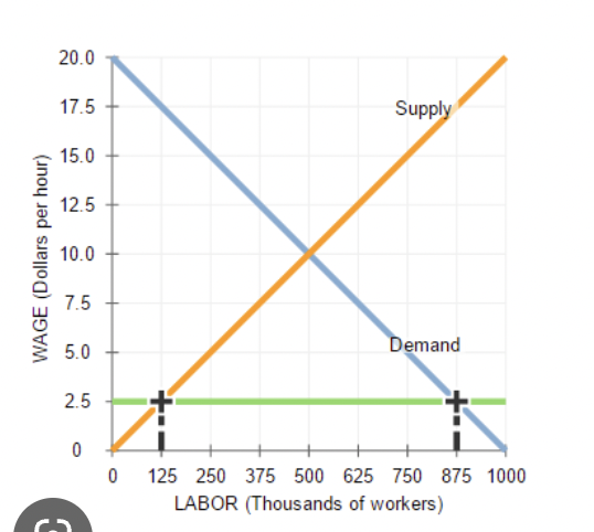
The next graph is a shortage of labor caused by an artificially low wage. There aren't too many concrete examples of this in the real world, but a maximum wage imposed by the government would be an example. In the below graph, we have a low wage of $2.50. This means firms demand 875 workers but only 125 workers are willing to sell their labor at that low wage.
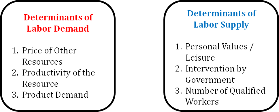
Determinants of Factor Demand
There are three components of resource demand that will change the demand for the resources. We could refer to these as the determinants of resource demand.
Prices of Related Input
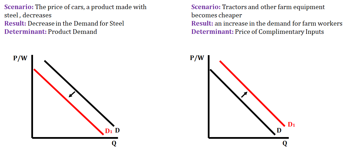
The first determinant is the price of related inputs. In this determinant, we are referring to substitute resources and complementary resources that are used in the production of goods and services. If the price of one resource becomes more expensive, the firm will increase their demand for the substitute resource. For example, if the price of copper piping increases, home builders will more willing to demand plastic piping. In looking at complementary resources, we can look at the production of soft drinks. Both aluminum and sugar are used in the production of soft drinks. If the price of aluminum increases, then we would see the demand for sugar decrease since both products are used to produce soft drinks.
Changes in Productivity
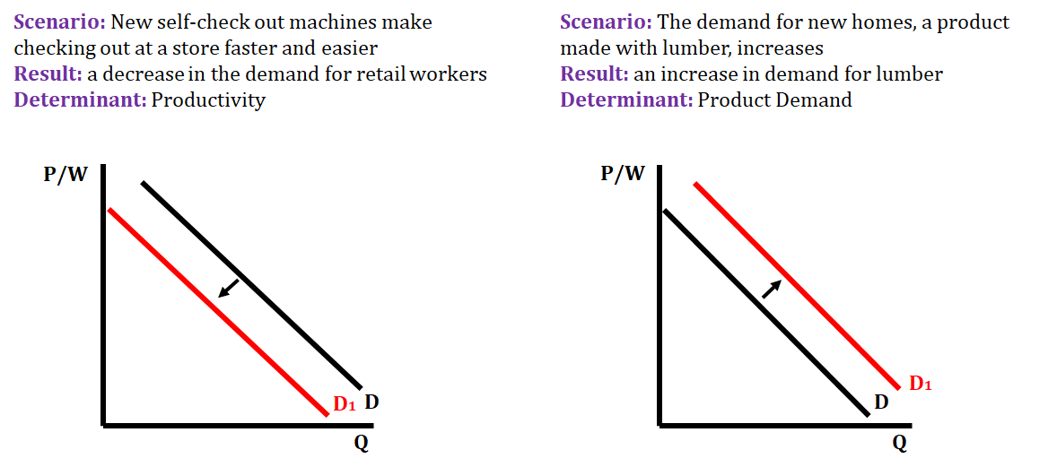
The second determinant of resource demand is a change in productivity. Let's take a situation where a new technique is developed that cuts production time in half. Since labor productivity has increased, each worker can make a greater quantity of the goods than they used to. This leads to each worker generating a greater marginal revenue product which increases their value to the firm or business. As a result, this increases the demand for labor.
Product Demand
The third determinant of resource demand is a change in the demand for the good or service. For example, if there is an increase in the demand for pizza, then there will be greater demand for all the resources that are involved in the production of pizza, including cheese, sauce, dough, and workers. Resource demand can also change when the price of a product changes. For example, if the price of pizza decreases, then the worker who is trained to make a pizza generates a smaller MRP (because MRP = MP x price), so the demand for these workers will decrease.
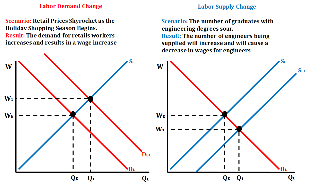
Let's look at some scenarios on graphs:
Determinants of Factor Supply
Just like with the demand for resources, there are several things that can change the supply of resources. When we are looking at the supply of resources, we generally focus on workers.
Number of Qualified Workers
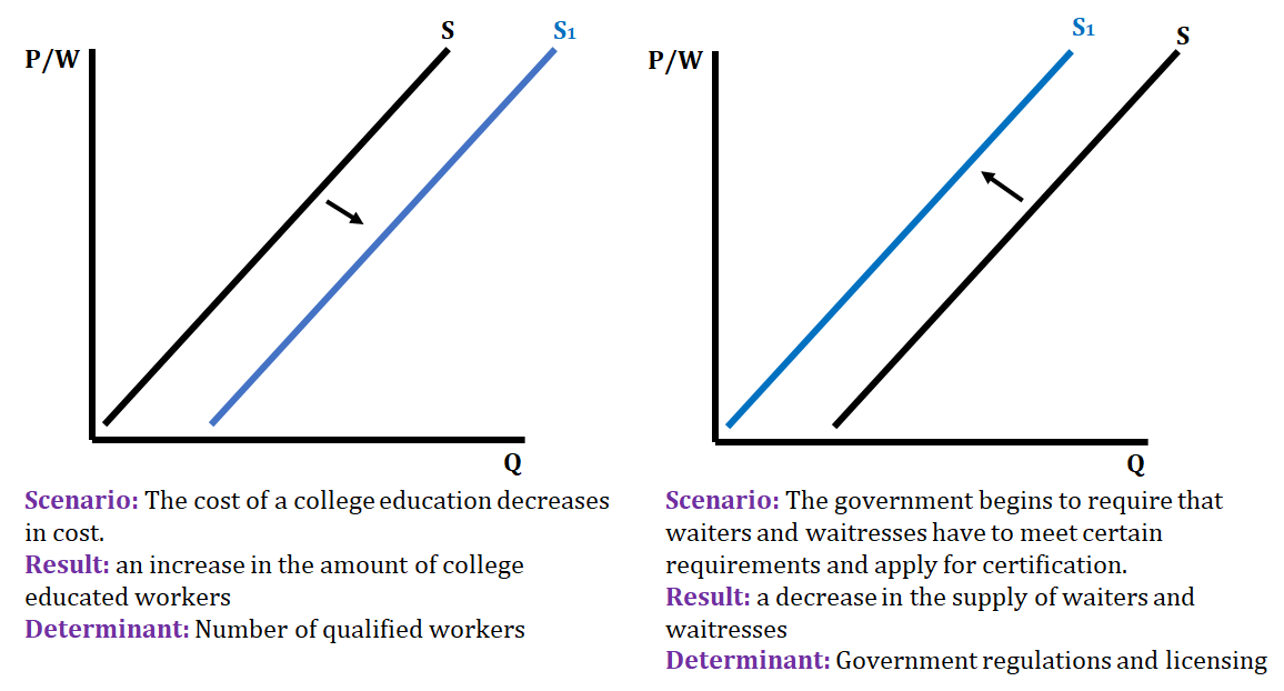
The first determinant of the supply of workers is the number of qualified workers that are available in a particular industry. This can be influenced by immigration, education, training, and abilities. Here are some examples of this determinant:
- If a country enacts stricter immigration laws than that will shift the labor supply to the left because of the smaller pool of workers.
- The number of graduates with engineering degrees soar. This would cause the labor supply to shift right.
Government Regulations
The second determinant of the supply of workers is government regulations and licensing. Here are some examples of this determinant:
- If the government establishes a certification process that makes it harder to be an electrician than we would see the supply of electricians decrease shifting the labor supply curve to the left.
Personal Values
The third determinant is personal values regarding leisure time and societal roles. Here are some examples of this determinant.
- The increase in the labor force, especially women, during WWII because people saw it as a patriotic duty to help produce the goods that would help in the war efforts. This would increase the labor supply and shift the curve right.
- Low-skill workers decide that working at minimum wage isn't worth their time. This would shift the labor supply curve to the left due to the decrease in the amount of workers.
- The wealth effect states that if long-term wealth increases, fewer people will supply labor at all wages, meaning supply shifts left, and vice-versa.
Let's look at some scenarios on graphs:
Changes in the Labor Market Equilibrium
Remember there are determinants that change both labor demand and labor supply. When these determinants occur, there is a change in the equilibrium of the labor market.
Let's look at an example that changes labor demand and an example that changes labor supply.
Frequently Asked Questions
What is factor demand and how is it different from regular demand?
Factor demand is the demand for an input (like labor) that’s derived from the demand for the final good it helps produce. Firms hire workers up to the point where the value of the marginal product of labor (VMPL or MRP = MPL × output price) equals the wage. Regular (consumer) demand is for final goods and reflects consumers’ direct valuations. Key differences: - Source: factor demand is derived from product demand; regular demand is direct. - Decision rule: firms hire where MRP = wage; consumers buy where marginal benefit = price. - Shifts: changes in output price or worker productivity shift labor demand (EK PRD-4.B.1); changes in tastes/income shift consumer demand. On the AP Micro FRQ you’ll often draw labor demand (MRP) and supply curves and show shifts (Topic 5.2). For a quick review, see the Fiveable study guide on this topic (https://library.fiveable.me/ap-microeconomics/unit-5/changes-factor-demand-factor-supply/study-guide/0IIdcKCqjk97CeKAPC0V) and more unit resources (https://library.fiveable.me/ap-microeconomics/unit-5).
How do I know when the labor demand curve shifts vs when there's just movement along the curve?
You get a movement along the labor demand curve when only the wage (price of labor) changes—firms hire more or less at different wages because the value of the marginal product (VMP = P × MPL or MRP) intersects the wage at a new point. The curve shifts when a determinant other than the wage changes. Per the CED, examples that shift labor demand: a change in the output price (P) or a change in worker productivity (MPL)—both change the VMP at every quantity, so the whole demand curve shifts right (increase) or left (decrease). Quick checklist to decide: Did the wage change? → movement along the curve. Did output price, technology/productivity, or demand for the product change? → shift of the labor demand curve. On AP free-response, draw and label the shift (PRD-4.B uses graphs)—show old and new demand curves and the new equilibrium wage and employment. For a short refresher, see the Topic 5.2 study guide (https://library.fiveable.me/ap-microeconomics/unit-5/changes-factor-demand-factor-supply/study-guide/0IIdcKCqjk97CeKAPC0V). For more practice problems, check Fiveable’s unit page (https://library.fiveable.me/ap-microeconomics/unit-5) and the practice question bank (https://library.fiveable.me/practice/ap-microeconomics).
What are the main things that cause labor demand to shift right or left?
Labor demand is derived from the value of marginal product (VMP = MPL × output price), so anything that raises or lowers MPL or the product’s price shifts the labor demand curve. Key causes that shift labor demand right (increase demand) - Higher output price (firms get more revenue per unit → VMP up) - Higher worker productivity (better tech, more human capital → MPL up) - More firms entering the industry (market demand for labor rises) - If a complementary input becomes cheaper and raises output, demand for labor can rise Key causes that shift labor demand left (decrease demand) - Lower output price - Falling worker productivity (worse tech, skill loss) - Fewer firms in the industry - If capital becomes cheaper and is a substitute for labor, firms may use more capital and less labor On the AP exam you’ll often show this with a right/left shift of the labor demand curve (Topic 5.2; relate to marginal revenue product). For a quick review, see the Topic 5.2 study guide (https://library.fiveable.me/ap-microeconomics/unit-5/changes-factor-demand-factor-supply/study-guide/0IIdcKCqjk97CeKAPC0V). For more practice, check unit resources (https://library.fiveable.me/ap-microeconomics/unit-5) and 1,000+ practice problems (https://library.fiveable.me/practice/ap-microeconomics).
I'm confused about how worker productivity affects labor demand - can someone explain this simply?
Short answer: higher worker productivity raises labor demand because each extra worker produces more value for the firm. In AP terms, a worker’s marginal product of labor (MPL) increases → marginal revenue product of labor (MRPL = MPL × price of output for a competitive firm) rises. Firms hire where MRPL = wage, so an upward change in MRPL shifts the labor demand curve right and increases equilibrium employment and (possibly) wages. The reverse happens if productivity falls. On the exam, show this with a correctly labeled graph: labor on x-axis, wage on y-axis, draw labor demand (MRPL) shifting right. This is EK PRD-4.B.1 territory and a skill often tested on free-response (you may be asked to draw and explain shifts). For a clear review, see the Topic 5.2 study guide (https://library.fiveable.me/ap-microeconomics/unit-5/changes-factor-demand-factor-supply/study-guide/0IIdcKCqjk97CeKAPC0V). For extra practice problems, check Fiveable’s practice bank (https://library.fiveable.me/practice/ap-microeconomics).
What's the difference between labor supply and labor demand shifts?
Labor demand and labor supply shifts are about different causes and directions on the same graph. Labor demand is a derived demand—firms hire workers because of the value those workers add (marginal revenue product of labor, MRP). Anything that raises MRP (higher output price, greater worker productivity/tech, more demand for the firm’s product) shifts the labor demand curve right; a fall in those shifts it left (EK PRD-4.B.1). Labor supply shifts come from changes in workers’ willingness or ability to work: immigration, education, preferences for leisure, working conditions, age distribution, or alternative options. Those move the labor supply curve right (more workers) or left (fewer workers) (EK PRD-4.B.2). On a graph, a rightward demand shift raises equilibrium wage and employment; a rightward supply shift lowers wage but raises employment. Practice drawing these for free-response (Topic 5.2 study guide: https://library.fiveable.me/ap-microeconomics/unit-5/changes-factor-demand-factor-supply/study-guide/0IIdcKCqjk97CeKAPC0V). For more unit review see (https://library.fiveable.me/ap-microeconomics/unit-5) and plenty of practice problems at (https://library.fiveable.me/practice/ap-microeconomics).
How does immigration affect the labor supply curve and which way does it shift?
Immigration increases the number of workers available, so it shifts the labor supply curve to the right (an increase in labor supply). On a standard labor-market graph (wage on vertical axis, quantity of labor on horizontal), S1 → S2. In a competitively supplied labor market that means the equilibrium wage falls (W1 → W2) and employment rises (L1 → L2). Use AP terms: this is a change in a determinant of labor supply (EK PRD-4.B.2), not a movement along the curve. You should be able to draw this shift on free-response graphs (Skill 4.C): show the supply curve moving right and label the new equilibrium wage and quantity. For more practice and examples tied to Topic 5.2, check the Fiveable study guide (https://library.fiveable.me/ap-microeconomics/unit-5/changes-factor-demand-factor-supply/study-guide/0IIdcKCqjk97CeKAPC0V) and Unit 5 overview (https://library.fiveable.me/ap-microeconomics/unit-5).
When the price of the output increases, what happens to the demand for workers and why?
If the output price rises, the value of the marginal product of labor (VMP or marginal revenue product, MRP = MPL × price) increases. That raises each worker’s contribution to revenue, so the firm’s labor demand curve (derived demand) shifts right—firms want more workers at every wage. On a graph you’d show the labor demand curve moving right and the equilibrium employment rising (until MRP = wage). This is EK PRD-4.B.1: a change in an output price shifts labor demand. For AP free-response expect to draw and label the shift and explain MRP rising; practice this on the Topic 5.2 study guide (https://library.fiveable.me/ap-microeconomics/unit-5/changes-factor-demand-factor-supply/study-guide/0IIdcKCqjk97CeKAPC0V). For extra practice problems, see (https://library.fiveable.me/practice/ap-microeconomics).
I don't understand how education levels change labor supply - help?
Short answer: Education changes labor supply by changing who’s available and what skills they offer. More education raises workers’ human capital → higher marginal product of labor and a higher value of marginal product (so firms demand more skilled labor). It also changes the supply curve for different skill groups: the supply of skilled workers shifts right (more people qualify for skilled jobs), while the supply of low-skilled labor can fall. Graphically, show separate labor markets (or separate curves for skilled vs. unskilled): higher education → rightward shift of the skilled labor supply and an upward/rightward shift of labor demand for skilled workers (higher MRP). Also note timing: more years of schooling delays entry into the workforce (short-run decrease in total labor supply), but long run increases skilled supply. For AP exam, be ready to draw labeled labor supply/demand curves and explain shifts (CED PRD-4.B.1 & 4.B.2). For more review, see the Topic 5.2 study guide (https://library.fiveable.me/ap-microeconomics/unit-5/changes-factor-demand-factor-supply/study-guide/0IIdcKCqjk97CeKAPC0V) and Unit 5 overview (https://library.fiveable.me/ap-microeconomics/unit-5). Practice problems: (https://library.fiveable.me/practice/ap-microeconomics).
What are all the determinants of labor supply that I need to memorize for the AP test?
Memorize the CED list—these are the determinants of labor supply that cause the labor supply curve to shift (EK PRD-4.B.2 / PRD-4.B): - Immigration (more workers → right shift; emigration → left) - Education/human capital (more skills → larger supply of qualified workers → right) - Working conditions and nonwage benefits (better conditions → attract more workers → right) - Age distribution of the population (more working-age people → right) - Availability of alternative options (e.g., more unemployment benefits or attractive other jobs → can reduce labor supply in a market → left) - Preferences for leisure vs. work (stronger preference for leisure → left) - Cultural expectations (norms about work participation, e.g., female labor force participation → shifts supply) On the exam you should be able to explain and show these shifts on a labor-supply/demand graph (PRD-4.B). Review Topic 5.2 study guide for examples (https://library.fiveable.me/ap-microeconomics/unit-5/changes-factor-demand-factor-supply/study-guide/0IIdcKCqjk97CeKAPC0V) and practice questions (https://library.fiveable.me/practice/ap-microeconomics).
How do I draw a graph showing both labor demand and supply shifting at the same time?
Draw one labor-market graph: wage (W) on the vertical axis and quantity of labor (L) on the horizontal. Start with a downward-sloping labor demand curve (MDP or VMP of L) and an upward-sloping labor supply curve (S). Label the initial equilibrium W0 and L0. To show simultaneous shifts: - If demand rises (e.g., higher output price or productivity), draw the demand curve rightward to D1 (MDP1). - If supply falls (e.g., emigration or more leisure preference), draw the supply curve leftward to S1. Mark the new intersection as W1 and L1. Show arrows on each curve indicating the direction of the shift. Interpretation: compare W1 vs W0 and L1 vs L0—wage could rise a lot if demand ↑ and supply ↓; employment change depends on relative shift sizes. On AP free-response, label curves, original and new equilibria, and briefly state the determinants causing each shift (CED EK PRD-4.B.1 and PRD-4.B.2). For a refresher and practice, see the Topic 5.2 study guide (https://library.fiveable.me/ap-microeconomics/unit-5/changes-factor-demand-factor-supply/study-guide/0IIdcKCqjk97CeKAPC0V) and Unit 5 overview (https://library.fiveable.me/ap-microeconomics/unit-5).
Why do better working conditions shift labor supply to the right?
Better working conditions (safer workplace, flexible hours, benefits) raise the non-wage utility of working. That means, for any given wage, more people are willing to work—or existing workers are willing to supply more hours. In CED terms this is a change in preferences/working conditions (one determinant of labor supply), so the labor supply curve shifts right. Think of it as a compensating-wage differential in reverse: if unpleasant jobs need higher pay to attract workers, improving conditions lowers the “wage premium” required, so supply increases at each wage. On an AP free-response graph, show the supply curve (S → S2) shifting right and label a larger quantity of labor demanded at the original wage. This connects to PRD-4.B and EK PRD-4.B.2—review the Topic 5.2 study guide for practice and examples (https://library.fiveable.me/ap-microeconomics/unit-5/changes-factor-demand-factor-supply/study-guide/0IIdcKCqjk97CeKAPC0V). For extra practice, try problems at (https://library.fiveable.me/practice/ap-microeconomics).
What happens to equilibrium wage and quantity when labor demand increases but supply stays the same?
If labor demand increases (the labor demand curve shifts right) while labor supply stays the same, the equilibrium wage rises and the equilibrium quantity of labor employed increases. That’s because firms’ derived demand for labor—driven by a higher value of the marginal product of labor or a higher output price—means at every wage firms want more workers. With an unchanged upward-sloping labor supply curve, the new intersection is at a higher wage and larger employment level. On the AP exam you should show this with a correctly labeled graph (wage on the vertical axis, quantity of labor on the horizontal) and explain using MRP = value of marginal product and derived demand (Skill 4.C / PRD-4.B). For review and practice problems, see the Topic 5.2 study guide (https://library.fiveable.me/ap-microeconomics/unit-5/changes-factor-demand-factor-supply/study-guide/0IIdcKCqjk97CeKAPC0V) and lots of practice at (https://library.fiveable.me/practice/ap-microeconomics).
Can someone explain how cultural expectations affect labor supply with a real world example?
Cultural expectations change people’s preferences for work versus leisure, so they shift the labor supply curve. For example, as cultural norms changed and more women chose paid work outside the home, the labor supply for many occupations increased—that’s a rightward shift in the labor supply curve (more workers willing to work at each wage). On a graph you’d show the supply curve moving right, lowering equilibrium wage and raising employment (holding demand constant). This is a change in determinants of labor supply (preferences/cultural expectations) from EK PRD-4.B.2; firms respond by hiring more because MRP of labor still determines demand. On the AP free-response you might be asked to draw this shift and explain the labor–leisure tradeoff. For a quick review and practice, check the Topic 5.2 study guide (https://library.fiveable.me/ap-microeconomics/unit-5/changes-factor-demand-factor-supply/study-guide/0IIdcKCqjk97CeKAPC0V) and more practice problems (https://library.fiveable.me/practice/ap-microeconomics).
I'm studying for FRQs - how do I know whether to talk about demand shifts or supply shifts in a labor market question?
Quick rule: ask “what changed that affects firms’ willingness to hire?” If it’s about output or how productive workers are (price of the good, tech that raises marginal product, or anything that changes the value of marginal product of labor/MRP), talk about a shift in labor demand (MRP curve shifts). If it’s about workers’ choices or availability (immigration, education, tastes for leisure, alternative jobs, working conditions), talk about a shift in labor supply. In FRQs you should: - Name the determinant (e.g., “increase in output price → demand for labor shifts right because VMP rises” or “large immigration → supply of labor shifts right”). - Draw labeled graphs showing the correct curve shift, new equilibrium wage and quantity, and explain the effect on wage/quantity using MRP or labor–leisure language. Remember graphing is a big FRQ chunk (graph/visual tasks count heavily on the exam). For examples, strategies, and practice FRQs, see the Topic 5.2 study guide (https://library.fiveable.me/ap-microeconomics/unit-5/changes-factor-demand-factor-supply/study-guide/0IIdcKCqjk97CeKAPC0V) and more practice at (https://library.fiveable.me/practice/ap-microeconomics).
What's the relationship between marginal revenue product and labor demand shifts?
Marginal revenue product (MRP) = marginal product of labor (MPL) × marginal revenue (MR). For a perfectly competitive firm MR = price, so the firm’s labor demand curve is its MRP curve—it hires where MRP = wage. That means any change that raises MRP at every L (like higher output price or greater worker productivity) shifts the labor demand curve right; the opposite shifts it left (EK PRD-4.B.1). Example: if output price rises 10% and productivity is unchanged, MR rises 10% so MRP rises 10% at each L and demand shifts right. In an imperfectly competitive firm MR falls with output, so MRP falls faster and the demand curve lies below the value of marginal product, but the logic for shifts is the same. On the AP exam you should show this with labeled graphs (shift right/left and new equilibrium wage/quantity)—that’s tested in FRQs (PRD-4.B). For a quick review see the Topic 5.2 study guide (https://library.fiveable.me/ap-microeconomics/unit-5/changes-factor-demand-factor-supply/study-guide/0IIdcKCqjk97CeKAPC0V) and more Unit 5 resources (https://library.fiveable.me/ap-microeconomics/unit-5). For extra practice problems, check Fiveable’s practice page (https://library.fiveable.me/practice/ap-microeconomics).