6.2 Constructing a Confidence Interval for a Population Proportion
7 min read•january 3, 2023
Josh Argo
Jed Quiaoit
Josh Argo
Jed Quiaoit
A is a range of values that is calculated from sample data and is used to estimate a . In the case of , a is used to estimate a . 🔸
The is based on the sample proportion, the sample size, and the of the sample size. The is the distribution of the sample statistic (in this case, the sample proportion) that would be obtained if we were to take multiple samples from the population and calculate the sample statistic for each sample.
The is a measure of how confident we are that the contains the true . In other words, our is reliant on a , which impacts how confident we are that our interval contains the true . The standard is usually 95%.
As the increases, the width of our interval also increases. ⬆️
Checking Conditions
Random Sample
This reduces any that may be caused from taking a bad sample. When answering inference questions, it is always essential to make note that our sample was random, either by highlighting text on the exam, or by quoting the problem where it details its randomness. Without a , our findings cannot be generalized to a population. This means that our scope of inference is inaccurate. There are no calculations that can fix an un-random, or biased, sample. 📚
Independence
This ensures that each subject in our sample was not influenced by the previous subjects chosen. While we are sampling without replacement, if our sample size is not super close to our population size, we can conclude that the effect it has on our sampling is negligible. We can check this condition by questioning if it is reasonable to believe that the population in question is at least 10 times as large as our sample. 🤔
For example, if we have a of 85 teenagers math grades and we are creating a for what the proportion of ALL teenagers passing their math class, we could state, "It is reasonable to believe that there are at least 850 teenagers currently enrolled in a math class."
To sum this idea up: When sampling without replacement, check that n ≤10%N, where N is the size of the population. A good way to state this when performing inference is to say, "It is reasonable to believe that our population (in context) is at least 10n." 💡
Normal
This check verifies that we are able to use a to calculate our probabilities using either or z scores. We can verify that a is normal using the Large Counts Condition, which states that we have at least 10 expected successes and 10 expected failures.
In the example listed above, let's say that we were given the proportion that 70% of all teenagers pass their math class. That means that with a sample of 85, 0.75(85)=63.75, which is greater than 10. We also have to check the complement by calculating 0.25(85)=21.25, which is also greater than 10.
Since both np and n(1-p) are greater than or equal to 10, we can conclude that the of our proportion will be approximately normal. 🎉
One Sample z-interval for Proportions
A one-sample z-interval for a proportion is an appropriate procedure for constructing a for a single based on a sample of . This procedure uses a z-test to estimate the based on the sample proportion and the sample size. 😳
The one-sample z-interval for a proportion is used when the following conditions are met:
The sample is a , or the sample size is large enough (usually n > 30) to use the normal approximation to the binomial distribution.
The data are collected from a single categorical variable, such as a yes/no response or a .
The sample size is large enough to use the normal approximation to the binomial distribution.
The is unknown and needs to be estimated from the sample data.
To construct a one-sample z-interval for a proportion, the sample proportion and sample size are used to calculate a z-score, which is then used to determine the . The is calculated as the sample proportion plus or minus a multiple of the . The is a measure of the variability of the sample proportion and is calculated using the sample size and the (which is assumed to be equal to the sample proportion).
Calculating the Interval
Calculating a is based on two things: our and our .
(1) Point Estimate
The for a used to estimate a is the sample proportion, which is also known as the p-hat. The sample proportion is the estimate of the based on the sample data.
The sample proportion is the middle point of the and is used to calculate the bounds. 📱
As you'll see later, the bounds are calculated by adding and subtracting a multiple of the to the sample proportion.
(2) Margin of Error
The is the "buffer zone" of the and is used to allow for the possibility of error or uncertainty in the estimate of the . his is what we add and subtract to our sample proportion to allow some room for error in our interval. The is a measure of the variability of the sample proportion and is calculated using the sample size and the (which is assumed to be equal to the sample proportion).
The is based on the critical value (z-score), which is a value that is determined by the , and the of the , and . The critical value is the number of standard deviations that the sample statistic is from the . For example, if the is 95%, the critical value is usually 1.96.
The sample size has a significant impact on the . As the sample size increases, the of the decreases, which results in a smaller . This means that as the sample size increases, the becomes narrower and the estimate of the becomes more precise. 🎯
Formula and Some Notes
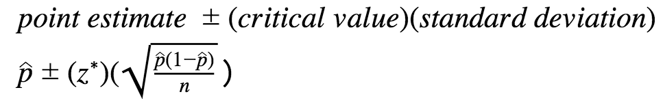
Note that the formula for the can be rearranged to solve for the minimum sample size needed to achieve a given . The formula for the is:
= z * , where z is the critical value and the is calculated using the sample size and the (which is assumed to be equal to the sample proportion).
To solve for the minimum sample size needed to achieve a given , we can rearrange the formula as follows:
n = (z / )^2 * p * (1 - p), where n is the minimum sample size, z is the critical value, is the desired , p is the (which is assumed to be equal to the sample proportion), and 1 - p is the of the other category.
If you are trying to find an upper bound for the sample size, you can use a guess for p or use p = 0.5 in order to find the maximum sample size that will result in a given . This will give you an idea of the maximum sample size that you would need in order to achieve the desired . ❤️
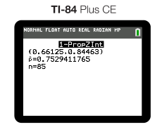
Using a Calculator
A much easier, more efficient way of calculating a is to use a graphing calculator or other form of technology. When using a graphing calculator such as a Texas Instruments TI-84, you would select 1-Prop Z Interval from the Stats menu, enter your number of successes (x), sample size (n), and . Lastly, calculate and you will get the you requested! 🖥️
🎥 Watch: AP Stats - Inference: Confidence Intervals for Proportions
Key Terms to Review (18)
Bias
: Bias refers to a systematic deviation from the true value or an unfair influence that affects the results of statistical analysis. It can occur during data collection, sampling, or analysis and leads to inaccurate or misleading conclusions.Categorical Data
: Categorical data refers to data that can be divided into categories or groups based on qualitative characteristics.Confidence Interval
: A confidence interval is a range of values that is likely to contain the true value of a population parameter. It provides an estimate along with a level of confidence about how accurate the estimate is.Confidence Level
: Confidence level refers to how confident we are that our interval estimate contains or captures the true population parameter. It represents our degree of certainty or reliability in estimating this parameter.Critical Value (z-score)
: The critical value, often represented as a z-score, is the number of standard deviations away from the mean that corresponds to a specific level of confidence in a hypothesis test or confidence interval.Dichotomous Variable
: A dichotomous variable is a categorical variable that can only take on two possible values or categories. It divides the data into two mutually exclusive groups.Empirical Rule
: The empirical rule, also known as the 68-95-99.7 rule, is a statistical guideline that states that for a normal distribution, approximately 68% of the data falls within one standard deviation of the mean, about 95% falls within two standard deviations, and roughly 99.7% falls within three standard deviations.Independence
: Independence refers to events or variables that do not influence each other. If two events are independent, knowing one event occurred does not affect our knowledge about whether or not the other event will occur.Margin of Error
: The margin of error is a measure of the uncertainty or variability in survey results. It represents the range within which the true population parameter is likely to fall.Normal Curve
: The normal curve (also known as bell curve) is a symmetrical distribution that represents many natural phenomena. It follows a specific mathematical pattern where most values cluster around the mean and progressively fewer values occur further away from the mean.p-hat (sample proportion)
: p-hat is the estimated proportion of a population based on a sample. It represents the ratio of successes to the total number of observations in the sample.Point Estimate
: A point estimate is a single value that is used to estimate an unknown population parameter. It is obtained from sample data and serves as our best guess for the true value of the parameter.Population Parameter
: A population parameter is a numerical value that describes a characteristic of an entire population.Population Proportion
: The population proportion refers to the proportion or percentage of individuals in a population who possess a specific characteristic or attribute. It represents the parameter of interest when studying categorical data.Random Sample
: A random sample is a subset of individuals selected from a larger population in such a way that every individual has an equal chance of being chosen. It helps to ensure that the sample is representative of the population.Sampling Distribution
: A sampling distribution refers to the distribution of a statistic (such as mean, proportion, or difference) calculated from multiple random samples taken from the same population. It provides information about how sample statistics vary from sample to sample.Standard Deviation
: The standard deviation measures the average amount of variation or dispersion in a set of data. It tells us how spread out the values are from the mean.Standard Error of the Proportion
: The standard error of the proportion measures the variability or uncertainty associated with estimating a population proportion from sample data. It quantifies how much we expect sample proportions to vary if we were to repeat the sampling process multiple times.6.2 Constructing a Confidence Interval for a Population Proportion
7 min read•january 3, 2023
Josh Argo
Jed Quiaoit
Josh Argo
Jed Quiaoit
A is a range of values that is calculated from sample data and is used to estimate a . In the case of , a is used to estimate a . 🔸
The is based on the sample proportion, the sample size, and the of the sample size. The is the distribution of the sample statistic (in this case, the sample proportion) that would be obtained if we were to take multiple samples from the population and calculate the sample statistic for each sample.
The is a measure of how confident we are that the contains the true . In other words, our is reliant on a , which impacts how confident we are that our interval contains the true . The standard is usually 95%.
As the increases, the width of our interval also increases. ⬆️
Checking Conditions
Random Sample
This reduces any that may be caused from taking a bad sample. When answering inference questions, it is always essential to make note that our sample was random, either by highlighting text on the exam, or by quoting the problem where it details its randomness. Without a , our findings cannot be generalized to a population. This means that our scope of inference is inaccurate. There are no calculations that can fix an un-random, or biased, sample. 📚
Independence
This ensures that each subject in our sample was not influenced by the previous subjects chosen. While we are sampling without replacement, if our sample size is not super close to our population size, we can conclude that the effect it has on our sampling is negligible. We can check this condition by questioning if it is reasonable to believe that the population in question is at least 10 times as large as our sample. 🤔
For example, if we have a of 85 teenagers math grades and we are creating a for what the proportion of ALL teenagers passing their math class, we could state, "It is reasonable to believe that there are at least 850 teenagers currently enrolled in a math class."
To sum this idea up: When sampling without replacement, check that n ≤10%N, where N is the size of the population. A good way to state this when performing inference is to say, "It is reasonable to believe that our population (in context) is at least 10n." 💡
Normal
This check verifies that we are able to use a to calculate our probabilities using either or z scores. We can verify that a is normal using the Large Counts Condition, which states that we have at least 10 expected successes and 10 expected failures.
In the example listed above, let's say that we were given the proportion that 70% of all teenagers pass their math class. That means that with a sample of 85, 0.75(85)=63.75, which is greater than 10. We also have to check the complement by calculating 0.25(85)=21.25, which is also greater than 10.
Since both np and n(1-p) are greater than or equal to 10, we can conclude that the of our proportion will be approximately normal. 🎉
One Sample z-interval for Proportions
A one-sample z-interval for a proportion is an appropriate procedure for constructing a for a single based on a sample of . This procedure uses a z-test to estimate the based on the sample proportion and the sample size. 😳
The one-sample z-interval for a proportion is used when the following conditions are met:
The sample is a , or the sample size is large enough (usually n > 30) to use the normal approximation to the binomial distribution.
The data are collected from a single categorical variable, such as a yes/no response or a .
The sample size is large enough to use the normal approximation to the binomial distribution.
The is unknown and needs to be estimated from the sample data.
To construct a one-sample z-interval for a proportion, the sample proportion and sample size are used to calculate a z-score, which is then used to determine the . The is calculated as the sample proportion plus or minus a multiple of the . The is a measure of the variability of the sample proportion and is calculated using the sample size and the (which is assumed to be equal to the sample proportion).
Calculating the Interval
Calculating a is based on two things: our and our .
(1) Point Estimate
The for a used to estimate a is the sample proportion, which is also known as the p-hat. The sample proportion is the estimate of the based on the sample data.
The sample proportion is the middle point of the and is used to calculate the bounds. 📱
As you'll see later, the bounds are calculated by adding and subtracting a multiple of the to the sample proportion.
(2) Margin of Error
The is the "buffer zone" of the and is used to allow for the possibility of error or uncertainty in the estimate of the . his is what we add and subtract to our sample proportion to allow some room for error in our interval. The is a measure of the variability of the sample proportion and is calculated using the sample size and the (which is assumed to be equal to the sample proportion).
The is based on the critical value (z-score), which is a value that is determined by the , and the of the , and . The critical value is the number of standard deviations that the sample statistic is from the . For example, if the is 95%, the critical value is usually 1.96.
The sample size has a significant impact on the . As the sample size increases, the of the decreases, which results in a smaller . This means that as the sample size increases, the becomes narrower and the estimate of the becomes more precise. 🎯
Formula and Some Notes
Note that the formula for the can be rearranged to solve for the minimum sample size needed to achieve a given . The formula for the is:
= z * , where z is the critical value and the is calculated using the sample size and the (which is assumed to be equal to the sample proportion).
To solve for the minimum sample size needed to achieve a given , we can rearrange the formula as follows:
n = (z / )^2 * p * (1 - p), where n is the minimum sample size, z is the critical value, is the desired , p is the (which is assumed to be equal to the sample proportion), and 1 - p is the of the other category.
If you are trying to find an upper bound for the sample size, you can use a guess for p or use p = 0.5 in order to find the maximum sample size that will result in a given . This will give you an idea of the maximum sample size that you would need in order to achieve the desired . ❤️
Using a Calculator
A much easier, more efficient way of calculating a is to use a graphing calculator or other form of technology. When using a graphing calculator such as a Texas Instruments TI-84, you would select 1-Prop Z Interval from the Stats menu, enter your number of successes (x), sample size (n), and . Lastly, calculate and you will get the you requested! 🖥️
🎥 Watch: AP Stats - Inference: Confidence Intervals for Proportions
Key Terms to Review (18)
Bias
: Bias refers to a systematic deviation from the true value or an unfair influence that affects the results of statistical analysis. It can occur during data collection, sampling, or analysis and leads to inaccurate or misleading conclusions.Categorical Data
: Categorical data refers to data that can be divided into categories or groups based on qualitative characteristics.Confidence Interval
: A confidence interval is a range of values that is likely to contain the true value of a population parameter. It provides an estimate along with a level of confidence about how accurate the estimate is.Confidence Level
: Confidence level refers to how confident we are that our interval estimate contains or captures the true population parameter. It represents our degree of certainty or reliability in estimating this parameter.Critical Value (z-score)
: The critical value, often represented as a z-score, is the number of standard deviations away from the mean that corresponds to a specific level of confidence in a hypothesis test or confidence interval.Dichotomous Variable
: A dichotomous variable is a categorical variable that can only take on two possible values or categories. It divides the data into two mutually exclusive groups.Empirical Rule
: The empirical rule, also known as the 68-95-99.7 rule, is a statistical guideline that states that for a normal distribution, approximately 68% of the data falls within one standard deviation of the mean, about 95% falls within two standard deviations, and roughly 99.7% falls within three standard deviations.Independence
: Independence refers to events or variables that do not influence each other. If two events are independent, knowing one event occurred does not affect our knowledge about whether or not the other event will occur.Margin of Error
: The margin of error is a measure of the uncertainty or variability in survey results. It represents the range within which the true population parameter is likely to fall.Normal Curve
: The normal curve (also known as bell curve) is a symmetrical distribution that represents many natural phenomena. It follows a specific mathematical pattern where most values cluster around the mean and progressively fewer values occur further away from the mean.p-hat (sample proportion)
: p-hat is the estimated proportion of a population based on a sample. It represents the ratio of successes to the total number of observations in the sample.Point Estimate
: A point estimate is a single value that is used to estimate an unknown population parameter. It is obtained from sample data and serves as our best guess for the true value of the parameter.Population Parameter
: A population parameter is a numerical value that describes a characteristic of an entire population.Population Proportion
: The population proportion refers to the proportion or percentage of individuals in a population who possess a specific characteristic or attribute. It represents the parameter of interest when studying categorical data.Random Sample
: A random sample is a subset of individuals selected from a larger population in such a way that every individual has an equal chance of being chosen. It helps to ensure that the sample is representative of the population.Sampling Distribution
: A sampling distribution refers to the distribution of a statistic (such as mean, proportion, or difference) calculated from multiple random samples taken from the same population. It provides information about how sample statistics vary from sample to sample.Standard Deviation
: The standard deviation measures the average amount of variation or dispersion in a set of data. It tells us how spread out the values are from the mean.Standard Error of the Proportion
: The standard error of the proportion measures the variability or uncertainty associated with estimating a population proportion from sample data. It quantifies how much we expect sample proportions to vary if we were to repeat the sampling process multiple times.Resources
© 2024 Fiveable Inc. All rights reserved.
AP® and SAT® are trademarks registered by the College Board, which is not affiliated with, and does not endorse this website.